Python API for the pycmplot package
Installation
Follow instructions in https://pypi.org/project/pycmplot/
Import the package functions
Eight main functions are involved in generating plots
prep_pycmplot_input_info: formats input streams correctly for data processing function–> auto-detects chrom, pos, snp, pval, and build columns
–> auto-detects delimiter
–> returns a dictionary with these information that the function below needs to appropriately handle sumstats.
get_sumstats_and_merged_sector_list: processes sumstat for plotting functions (work horse of the package)–> trims variants based on
trim_pvalthreshold to increase speed and memory efficiency of plotting functions–> fixes chrom labels
–> adds logP column if specified
–> adds a LABEL column which is simply the labels provided by user.
–> converts hg19 to hg38 genome build
–> identifies lead SNPs based on significance threshold and generates hits table
–> generates sector size dictionary for circular plots
–> generates dictionary of genome-wide significance and suggestive thresholds per summary stat
–> returns a pycmplot_dict dictionary containing input information for plotting functions. These include (these are the dict keys):
sectors: a dictionary of sector sizes for circular plotting.
dfs: the loaded summary stats with
trim_pvalapplied if set.annot: a hits summary table generated for potential annotation.
lines: a dictionary of values to use to plot genome-wide significance and suggestive lines.
pvals: a dictionary of raw p-values extracted for qq-plotting before applying
trim_pvalfor Manhattan plotting.
plot_linear: generates linear Manhattan plots–> returns plt.Axes
plot_circular: generates circular Manhattan plotsplot_qq_single: generates a qq-plot in user-supplied axis.Useful in creating customized multi-panel qq-plots in one figure.
–> returns plt.Axes
plot_qq_separate: generates separate qq-plots per sumstat in different figures.plot_qq_overlay: generates qq-plots in one figures on a single shared axes with different colors per sumstat, and lambda values included in legend.plot_qq_combined: generates multi-panel qq-plots usingplot_qq_singlearranged in a configurable column grid in a single figure.
NB: > Auto-detection of column names and delimiter is very important when dealing with multiple sumstats from different projects or tools with different > column naming styles.
[1]:
from pycmplot import (
    prep_pycmplot_input_info,
    get_sumstats_and_merged_sector_list,
    plot_linear, plot_circular,
    plot_qq_single,
    plot_qq_separate,
    plot_qq_overlay,
    plot_qq_combined,
)
Getting help
To see the options of a function, simply run help(function_name)
Example:
help(prep_pycmplot_input_info)
Example plotting
Prepare lists of your summary stats and their corresponding labels
[6]:
sumstats_list = [
    '/data/awonkam1/kesoh/gwas/sitt/sumher/pycmplot/sitt_all_panels_nHbF_agecut-5_kvik1.step2.assoc.gz',
    '/data/awonkam1/kesoh/gwas/sitt/sumher/pycmplot/sitt_all_panels_nMCV_agecut-5_kvik1.step2.assoc.gz'
]
labels_list = ['HbF','MCV']
Pass these lists to the
prep_pycmplot_input_infofunctionThese files include summary stats from multiple imputation panels in different genomic coordinates concatenated together and a column ‘BUILD’ added to indicate the build of each position
[3]:
sumstat_info_dict = prep_pycmplot_input_info(
    sum_stats=sumstats_list,
    labels=labels_list
)

# take a look at the dictionary: the function has auto-detected column names and delimiter
sumstat_info_dict
[3]:
{'HbF': [['CHR', 'POS', 'SNP', 'P', 'BUILD'],
  {'CHR': 'category',
   'POS': object,
   'SNP': str,
   'P': float,
   'BUILD': 'category'},
  {'CHR': 'CHR', 'POS': 'POS', 'SNP': 'SNP', 'P': 'P', 'BUILD': 'BUILD'},
  '\t'],
 'MCV': [['CHR', 'POS', 'SNP', 'P', 'BUILD'],
  {'CHR': 'category',
   'POS': object,
   'SNP': str,
   'P': float,
   'BUILD': 'category'},
  {'CHR': 'CHR', 'POS': 'POS', 'SNP': 'SNP', 'P': 'P', 'BUILD': 'BUILD'},
  '\t']}
Important notes
Hits table will be generated here containing variants and their gene annotations at the set significance threshold using the
signific_thresholdoption.If say you use a different p-value threshold to highlight positions in the plotting functions, those positions will be highlighted but will not be annotated because annotations in the
hits_tablewere generated using a different p-value threshold.If you wish to annotate all highlighted positions, then use the same
signif_thresholdandhighlight_thresholdeverywhere.For instance, below we use the default genome-wide significance threshold by not setting any value
[4]:
%%time
pycmplot_dict = get_sumstats_and_merged_sector_list(
    sum_stats=sumstats_list,
    labels=labels_list,
    file_info=sumstat_info_dict,
    logp=True,
    table_out="test_pycmplot_python_api",
    trim_pval=0.01
)

merged_assoc_sector_sizes = pycmplot_dict["sectors"]
sumstats_loaded = pycmplot_dict["dfs"]
hits_table = pycmplot_dict["annot"]
signif_lines = pycmplot_dict["lines"]
pval_dict = pycmplot_dict["pvals"]

hits_table
[INFO] Loading MCV from /data/awonkam1/kesoh/gwas/sitt/sumher/pycmplot/sitt_all_panels_nMCV_agecut-5_kvik1.step2.assoc.gz …
[INFO] Loaded 82710042 variants from summary stat file, using 6.84 GB of memory
[INFO] Extracting raw p-values for QQ-plotting ...
[INFO] Excluding variants with p-value less than 0.01 to speed up Manhattan plotting ...
[INFO] 854187 variants remain after trimming, using 7.74 MB of memory
[INFO] Adding a 'logP' column ...
[INFO] Normalizing chromosome names {"23": "X", "24": "Y", "M": "MT", "MTDNA": "MT"} ...
[INFO] Converting hg19 coordinates to hg38 ...
[INFO] Loading LiftOver chain file: /home/kesohku1/projects/gwas/scripts/pycmplot/pycmplot/data/hg19ToHg38.over.chain.gz
[INFO] Extracting variants to highlight ...
[INFO] Loading HbF from /data/awonkam1/kesoh/gwas/sitt/sumher/pycmplot/sitt_all_panels_nHbF_agecut-5_kvik1.step2.assoc.gz …
[INFO] Loaded 82710042 variants from summary stat file, using 6.84 GB of memory
[INFO] Extracting raw p-values for QQ-plotting ...
[INFO] Excluding variants with p-value less than 0.01 to speed up Manhattan plotting ...
[INFO] 890427 variants remain after trimming, using 8.07 MB of memory
[INFO] Adding a 'logP' column ...
[INFO] Normalizing chromosome names {"23": "X", "24": "Y", "M": "MT", "MTDNA": "MT"} ...
[INFO] Converting hg19 coordinates to hg38 ...
[INFO] Extracting variants to highlight ...
[INFO] Loading gene info from: /home/kesohku1/projects/gwas/scripts/pycmplot/pycmplot/data/Homo_sapiens.GRCh38.geneinfo.tsv.gz
[INFO] Annotating lead variants and generating hits summary table ...
[INFO] Locus summary written to: test_pycmplot_python_api.tsv
[INFO] Computing per-sumstat sector sizes (chrom → [min_pos, max_pos])
CPU times: user 4min 26s, sys: 22.6 s, total: 4min 49s
Wall time: 4min 50s
[4]:
| CHR | POS | SNP | P | BUILD | logP | LABEL | OLD_POS | OLD_BUILD | genic | ... | promoter_upstream_flag | gene_density | top_gene | biotype | priority_score | distance | promoter_flag | distance_score | biotype_weight | promoter_bonus | |
|---|---|---|---|---|---|---|---|---|---|---|---|---|---|---|---|---|---|---|---|---|---|
| 1 | 2 | 60493111 | 2:60493111:SNV | 3.039700e-18 | hg38 | 17.517169 | HbF | 60493111 | hg38 | True | ... | False | 46 | BCL11A | protein_coding | 4.0 | 0 | False | 1.0 | 1.0 | 0.0 |
| 0 | 16 | 258003 | 16:258003:SNV | 1.094200e-13 | hg38 | 12.960903 | MCV | 258003 | hg38 | True | ... | False | 150 | FAM234A | protein_coding | 4.0 | 0 | False | 1.0 | 1.0 | 0.0 |
2 rows × 24 columns
Generating a linear plot
We use the results of the function above.
No highlighting of significant loci
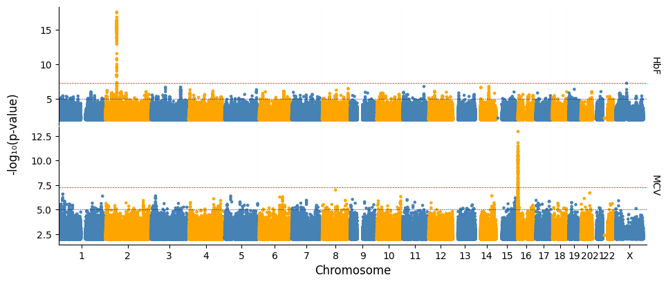
[5]:
%%time
axes = plot_linear(
    sumstats_loaded=sumstats_loaded,
    hits_table=hits_table,
    plot_title="test_pycmplot_python_api",
    output_format='png',
    dpi=300, chr_spacing=9e6,
    point_size=5, linear_track_spacing=0.01,
    signif_lines=signif_lines,
    logp=True, colors=['steelblue','orange'],
    figsize=(10, 4),
    trim_pval=0.001
)
[INFO] Plotting: HbF ...
[INFO] Plotting: MCV ...
[INFO] Saved linear Manhattan plot: /home/kesohku1/projects/gwas/scripts/pycmplot/testpycmplotpythonapi_hbf_mcv_lm_logp.png
CPU times: user 47.4 s, sys: 3.01 s, total: 50.4 s
Wall time: 48.5 s
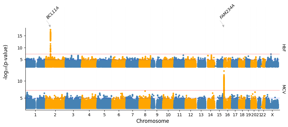
Generating a linear plot
Let’s include annotation
We will use the top_gene column of the hits table for annotation
We add an extra annotation track to
track_heights, the first value
[6]:
%%time
axes = plot_linear(
    sumstats_loaded=sumstats_loaded,
    track_heights=[0.5,1,1],
    hits_table=hits_table,
    plot_title="test_pycmplot_python_api",
    annotate='gene',
    #label_col='top_gene',
    output_format='png',
    dpi=300, chr_spacing=9e6, linear_track_spacing=0.02,
    point_size=8,
    signif_lines=signif_lines,
    logp=True, colors=['steelblue','orange'],
    figsize=(10, 4),
    trim_pval=0.001
)
[INFO] Annotate by: nearest_upstream_gene
[INFO] Plotting: HbF ...
[INFO] Plotting: MCV ...
[INFO] Saved linear Manhattan plot: /home/kesohku1/projects/gwas/scripts/pycmplot/testpycmplotpythonapi_hbf_mcv_lm_logp.png
CPU times: user 49 s, sys: 3.13 s, total: 52.1 s
Wall time: 50.3 s
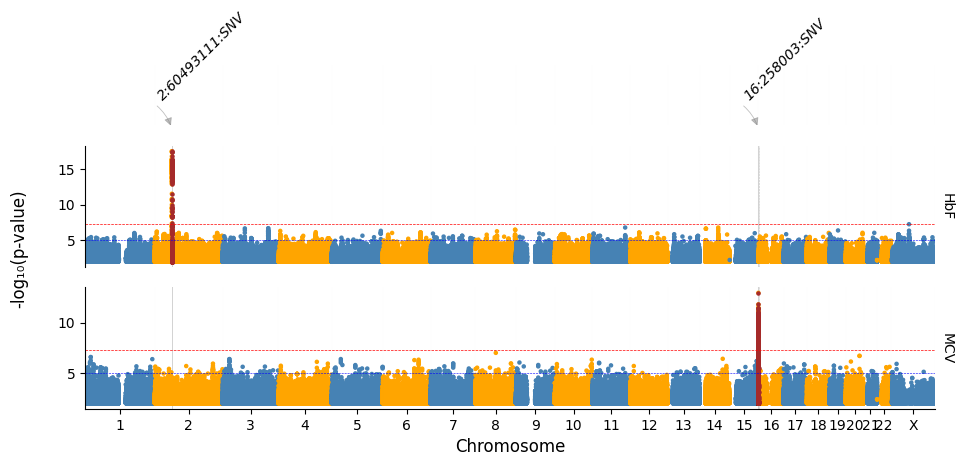
Highlighting significant loci and annotating by SNP
[7]:
%%time
axes = plot_linear(
    sumstats_loaded=sumstats_loaded,
    track_heights=[0.5,1,1],
    hits_table=hits_table,
    plot_title="test_pycmplot_python_api",
    annotate='SNP',
    output_format='png',
    dpi=300, chr_spacing=0.0,
    point_size=5,
    signif_lines=signif_lines,
    highlight=True,
    highlight_color="brown",
    highlight_line=True,
    highlight_line_color="lightgrey",
    logp=True, colors=['steelblue','orange'],
    figsize=(10, 4),
    trim_pval=0.001
)
[INFO] Annotate by: SNP
[INFO] Plotting: HbF ...
[INFO] Plotting: MCV ...
[INFO] Saved linear Manhattan plot: /home/kesohku1/projects/gwas/scripts/pycmplot/testpycmplotpythonapi_hbf_mcv_lm_logp.png
CPU times: user 50.9 s, sys: 3.81 s, total: 54.7 s
Wall time: 52.5 s
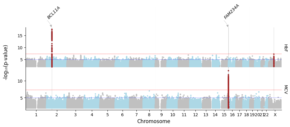
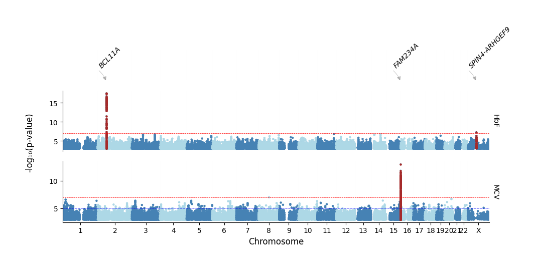
Highlighting by a different p-value threshold and changing plot colors and removing track labels
Notice that a chrX locus is highlighted but not annotated.
This is because it did not meat the default significance threshold used in the data preparation function that generated the hits table.
[8]:
%%time
axes = plot_linear(
    sumstats_loaded=sumstats_loaded,
    track_heights=[0.5,1,1], linear_track_spacing=0.01,
    hits_table=hits_table,
    plot_title="test_pycmplot_python_api",
    annotate='gene',
    label_col='top_gene',
    output_format='png',
    dpi=300, chr_spacing=0.01,
    point_size=5,
    signif_lines=signif_lines,
    highlight=True,
    highlight_thresh=1e-7,
    highlight_color="brown",
    highlight_line=True,
    highlight_line_color="lightgrey",
    logp=True, colors=['silver','lightblue'],
    figsize=(10, 4),
    trim_pval=0.001
)
[INFO] Annotate by: nearest_upstream_gene
[INFO] Plotting: HbF ...
[INFO] Plotting: MCV ...
[INFO] Saved linear Manhattan plot: /home/kesohku1/projects/gwas/scripts/pycmplot/testpycmplotpythonapi_hbf_mcv_lm_logp.png
CPU times: user 50.8 s, sys: 3.63 s, total: 54.4 s
Wall time: 52.2 s
Generating circular plots
Here, we specify gene annotation by the
annotateargument.It takes either
SNPorGENE. WhenGENEis specified, thetop_genecolumn in the hits table will be used.
[9]:
%%time
fig = plot_circular(
    sumstats_loaded=sumstats_loaded,
    hits_table=hits_table,
    sector_sizes=merged_assoc_sector_sizes,
    annotate="GENE",
    plot_title="Large Inner Circle: r_min = 40",
    #label_col='top_gene',
    output_format='png',
    annotation_size=10,
    dpi=300,
    highlight=True,
    pad=1,
    r_min=40,
    r_max=100,
    signif_lines=signif_lines,
    logp=True, colors=['steelblue','orange'],
    #figsize=(10, 4),
)
[INFO] Plotting : HbF
[INFO] Plotting : MCV
[INFO] Annotate by: nearest_upstream_gene
[INFO] Saved circular Manhattan plot: /home/kesohku1/projects/gwas/scripts/pycmplot/large_inner_circle_rmin__40_hbf_mcv_cm_logp.png
CPU times: user 1min 44s, sys: 3.84 s, total: 1min 48s
Wall time: 1min 46s
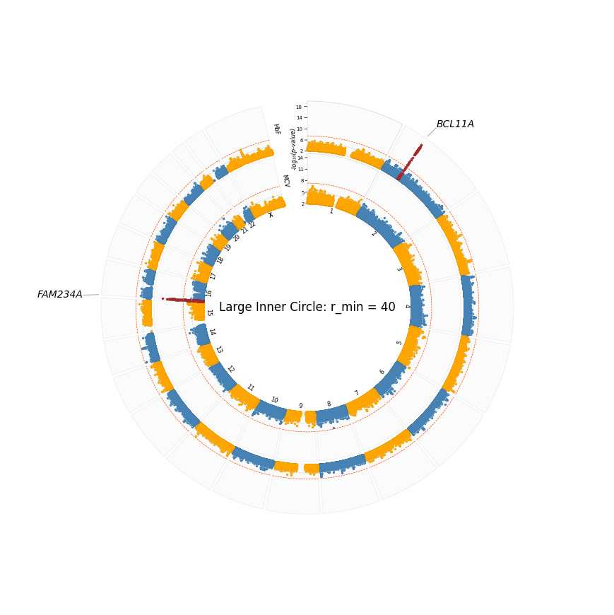
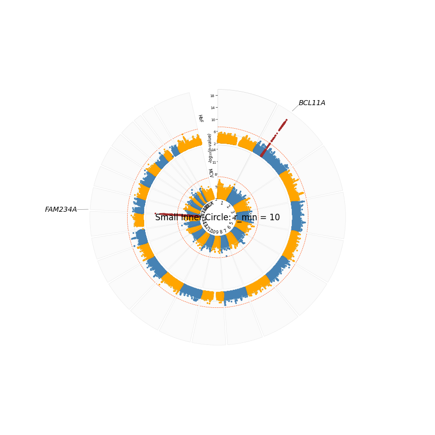
Controling the inner circle size
The inner circle size is controled by the
r_min(minimum radius) argument. It indicates the proportion of the figure the inner circle occupies.When dealing with a few sumstats, it should be appropriate to use a relatively high value so the tracks (Manhattan plots) a well represented.
With many more sumstats,
r_minshould be lower. For instance, I have noticed thatr_min = 20works well for >= 4 sumstats. 20 is thus the default whenr_minis not set.The total size of the circle is also determined by
r_max(maximum radius). It is recommended to always use the default of 100.For instance, we will use
r_min = 10below so you see that the plot looks messy with 2 sumstats.We can control the size of the plot title using
plot_title_size. However, anything fitted within that tiny space would not be visible.
[10]:
%%time
fig = plot_circular(
    sumstats_loaded=sumstats_loaded,
    hits_table=hits_table,
    sector_sizes=merged_assoc_sector_sizes,
    annotate="GENE",
    plot_title="Small Inner Circle: r_min = 10",
    #label_col='top_gene',
    output_format='png',
    annotation_size=10,
    dpi=300,
    highlight=True,
    pad=1,
    r_min=10,
    r_max=100,
    signif_lines=signif_lines,
    logp=True, colors=['steelblue','orange'],
    #figsize=(10, 4),
)
[INFO] Plotting : HbF
[INFO] Plotting : MCV
[INFO] Annotate by: nearest_upstream_gene
[INFO] Saved circular Manhattan plot: /home/kesohku1/projects/gwas/scripts/pycmplot/small_inner_circle_rmin__10_hbf_mcv_cm_logp.png
CPU times: user 1min 43s, sys: 4.1 s, total: 1min 48s
Wall time: 1min 45s
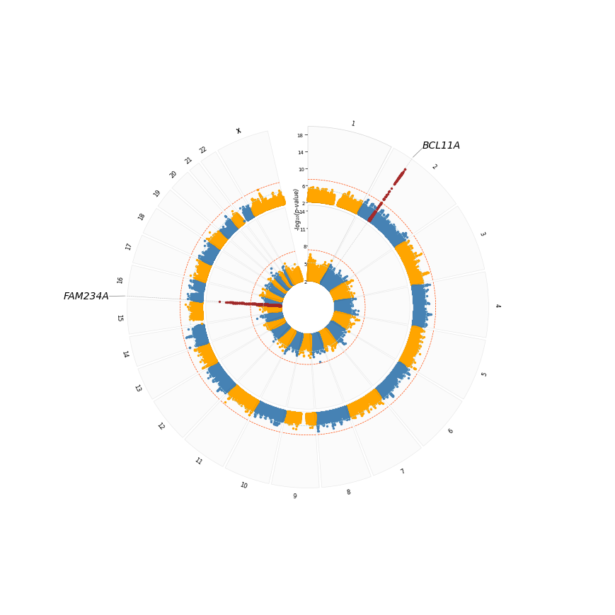
We can make it look better by placing chrom labels outside, and excluding plot title and track labels
[12]:
%%time
fig = plot_circular(
    sumstats_loaded=sumstats_loaded,
    hits_table=hits_table,
    sector_sizes=merged_assoc_sector_sizes,
    annotate="GENE",
    #plot_title="test_pycmplot_python_api",
    chrom_label_side='outside',
    output_format='png',
    annotation_size=10,
    dpi=300,
    highlight=True,
    highlight_line=True,
    no_track_labels=True,
    pad=1,
    r_min=10,
    r_max=100,
    signif_lines=signif_lines,
    logp=True, colors=['steelblue','orange'],
    #figsize=(10, 4),
)
[INFO] Plotting : HbF
[INFO] Plotting : MCV
[INFO] Annotate by: nearest_upstream_gene
[INFO] Saved circular Manhattan plot: /home/kesohku1/projects/gwas/scripts/pycmplot/dt4kk3raov_hbf_mcv_cm_logp.png
CPU times: user 1min 43s, sys: 3.54 s, total: 1min 47s
Wall time: 1min 45s
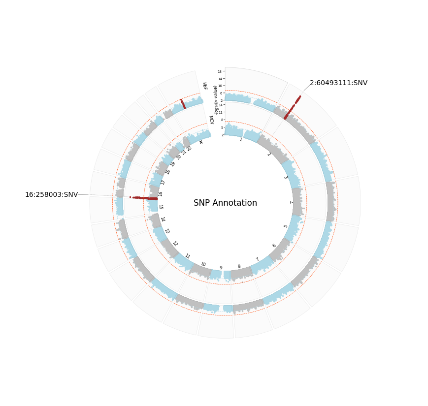
SNP Annotation, highlight threshold and color change
[11]:
%%time
fig = plot_circular(
    sumstats_loaded=sumstats_loaded,
    hits_table=hits_table,
    sector_sizes=merged_assoc_sector_sizes,
    annotate="SNP",
    plot_title="SNP Annotation",
    #label_col='top_gene',
    output_format='png',
    annotation_size=10,
    dpi=300,
    highlight=True,
    highlight_line=True,
    highlight_thresh=1e-7,
    pad=1,
    r_min=40,
    r_max=100,
    signif_lines=signif_lines,
    logp=True, colors=['silver','lightblue'],
    #figsize=(10, 4),
)
[INFO] Plotting : HbF
[INFO] Plotting : MCV
[INFO] Annotate by: SNP
[INFO] Saved circular Manhattan plot: /home/kesohku1/projects/gwas/scripts/pycmplot/snp_annotation_hbf_mcv_cm_logp.png
CPU times: user 1min 44s, sys: 3.71 s, total: 1min 48s
Wall time: 1min 46s
Ensuring all highlighted loci are also annotated
We set the same
signif_thresholdandhighlight_threshvalues.Remember you can give these outputs any name:
merged_sector_sizes,sumstats_loaded,hits_table,signif_lines
[13]:
%%time
pycmplot_dict = get_sumstats_and_merged_sector_list(
    sum_stats=sumstats_list,
    labels=labels_list,
    file_info=sumstat_info_dict,
    logp=True,
    table_out="test_pycmplot_python_api",
    trim_pval=0.001,
    signif_threshold=1e-7
)

merged_assoc_sector_sizes = pycmplot_dict["sectors"]
sumstats_loaded = pycmplot_dict["dfs"]
hits_table = pycmplot_dict["annot"]
signif_lines = pycmplot_dict["lines"]
pval_dict = pycmplot_dict["pvals"]

hits_table
[INFO] Loading MCV from /data/awonkam1/kesoh/gwas/sitt/sumher/pycmplot/sitt_all_panels_nMCV_agecut-5_kvik1.step2.assoc.gz …
[INFO] Loaded 82710042 variants from summary stat file, using 6.84 GB of memory
[INFO] Extracting raw p-values for QQ-plotting ...
[INFO] Excluding variants with p-value less than 0.001 to speed up Manhattan plotting ...
[INFO] 86296 variants remain after trimming, using 0.782 MB of memory
[INFO] Adding a 'logP' column ...
[INFO] Normalizing chromosome names {"23": "X", "24": "Y", "M": "MT", "MTDNA": "MT"} ...
[INFO] Converting hg19 coordinates to hg38 ...
[INFO] Extracting variants to highlight ...
[INFO] Loading HbF from /data/awonkam1/kesoh/gwas/sitt/sumher/pycmplot/sitt_all_panels_nHbF_agecut-5_kvik1.step2.assoc.gz …
[INFO] Loaded 82710042 variants from summary stat file, using 6.84 GB of memory
[INFO] Extracting raw p-values for QQ-plotting ...
[INFO] Excluding variants with p-value less than 0.001 to speed up Manhattan plotting ...
[INFO] 92724 variants remain after trimming, using 0.841 MB of memory
[INFO] Adding a 'logP' column ...
[INFO] Normalizing chromosome names {"23": "X", "24": "Y", "M": "MT", "MTDNA": "MT"} ...
[INFO] Converting hg19 coordinates to hg38 ...
[INFO] Extracting variants to highlight ...
[INFO] Loading gene info from: /home/kesohku1/projects/gwas/scripts/pycmplot/pycmplot/data/Homo_sapiens.GRCh38.geneinfo.tsv.gz
[INFO] Annotating lead variants and generating hits summary table ...
[INFO] Locus summary written to: test_pycmplot_python_api.tsv
[INFO] Computing per-sumstat sector sizes (chrom → [min_pos, max_pos])
CPU times: user 4min 13s, sys: 18.3 s, total: 4min 31s
Wall time: 4min 32s
[13]:
| CHR | POS | SNP | P | BUILD | logP | LABEL | OLD_POS | OLD_BUILD | genic | ... | promoter_upstream_flag | gene_density | top_gene | biotype | priority_score | distance | promoter_flag | distance_score | biotype_weight | promoter_bonus | |
|---|---|---|---|---|---|---|---|---|---|---|---|---|---|---|---|---|---|---|---|---|---|
| 1 | 2 | 60493111 | 2:60493111:SNV | 3.039700e-18 | hg38 | 17.517169 | HbF | 60493111 | hg38 | True | ... | False | 46.0 | BCL11A | protein_coding | 4.0 | 0 | False | 1.0 | 1.0 | 0.0 |
| 0 | 16 | 258003 | 16:258003:SNV | 1.094200e-13 | hg38 | 12.960903 | MCV | 258003 | hg38 | True | ... | False | 150.0 | FAM234A | protein_coding | 4.0 | 0 | False | 1.0 | 1.0 | 0.0 |
| 2 | X | 63094194 | 23:62313664:SNV | 5.633700e-08 | hg38 | 7.249206 | HbF | 62313664 | hg19 | False | ... | False | NaN | SPIN4-ARHGEF9 | intergenic | NaN | 253034-540773 | None | NaN | NaN | NaN |
3 rows × 24 columns
See that we now have three loci in the hits table
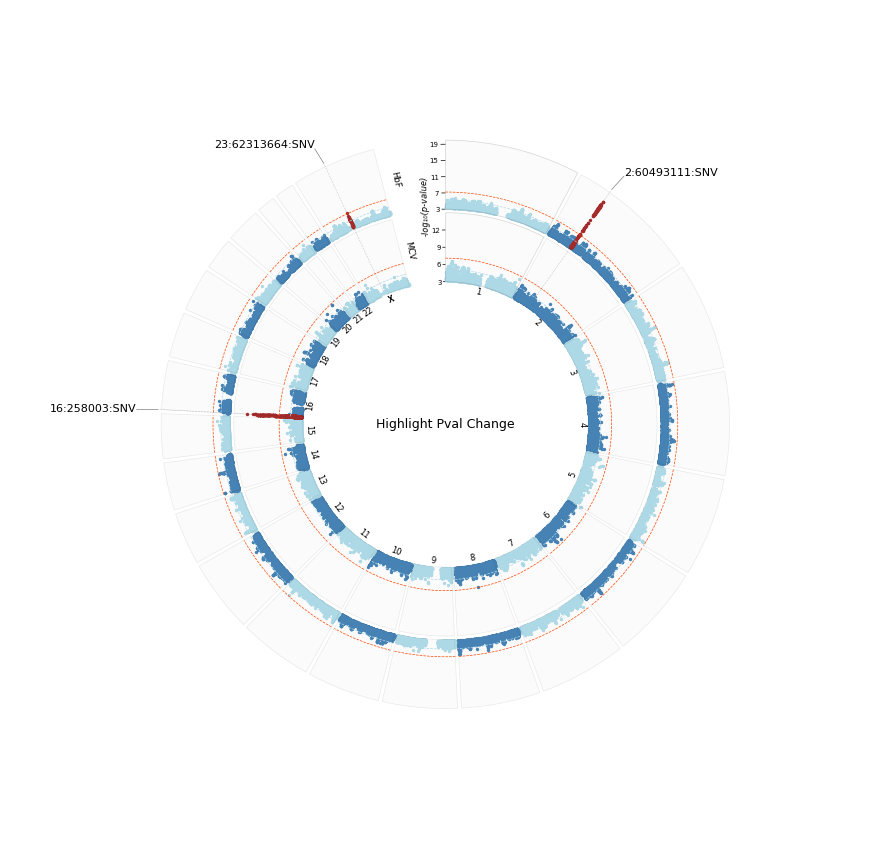
[5]:
%%time
fig1 = plot_circular(
    sumstats_loaded=sumstats_loaded,
    hits_table=hits_table,
    sector_sizes=merged_assoc_sector_sizes,
    annotate="GENE",
    plot_title="Highlight Pval Change",
    plot_title_size=9,
    #label_col='top_gene',
    output_format='png',
    annotation_size=8,
    dpi=300,
    highlight=True,
    highlight_thresh=1e-7,
    highlight_line=True,
    pad=1,
    r_min=40,
    r_max=100,
    signif_lines=signif_lines,
    logp=True, colors=['steelblue','lightblue'],
    #figsize=(10, 4),
)
[INFO] Plotting : HbF
[INFO] Plotting : MCV
[INFO] Saved circular Manhattan plot: /home/kesohku1/projects/gwas/scripts/pycmplot/highlight_pval_change_hbf_mcv_cm_logp.png
CPU times: user 15.8 s, sys: 1.37 s, total: 17.1 s
Wall time: 15.8 s
Explicitly speficying directory where output files should be stored
[7]:
%%time
axes = plot_linear(
    sumstats_loaded=sumstats_loaded,
    track_heights=[0.5,1,1],
    hits_table=hits_table,
    plot_title="test_pycmplot_python_api",
    output_dir='/home/kesohku1/projects/gwas/', # <--- output directory
    annotate=True,
    label_col='top_gene',
    output_format='png',
    dpi=300, chr_spacing=0.0,
    point_size=5,
    highlight=True,
    highlight_thresh=1e-7,
    signif_lines=signif_lines,
    logp=True, colors=['steelblue','lightblue'],
    figsize=(10, 4), # (with, height)
    trim_pval=0.001
)
[INFO] Plotting: HbF ...
[INFO] Plotting: MCV ...
[INFO] Saved linear Manhattan plot: /home/kesohku1/projects/gwas/testpycmplotpythonapi_hbf_mcv_lm_logp.png
CPU times: user 6.81 s, sys: 794 ms, total: 7.61 s
Wall time: 6.76 s
# Handling other use cases and QQ-plots
Summary stats without BUILD column and no build information provided
[2]:
# susmtats
sumstats_no_build_col_list = [
    "/data/awonkam1/kesoh/gwas/sitt/sumher/kgp/nHbF/kgp-r2-0.60-maf-0.01_nHbF_agecut-5_kvik1.step2.assoc.gz",
    "/data/awonkam1/kesoh/gwas/sitt/sumher/h3a/nMCV/h3a-r2-0.60-maf-0.01_nMCV_agecut-5_kvik1.step2.assoc.gz",
    "/data/awonkam1/kesoh/gwas/sitt/sumher/gmv2p1/nHb/gmv2p1-r2-0.60-maf-0.01_nHb_agecut-5_kvik1.step2.assoc.gz",
    "/data/awonkam1/kesoh/gwas/sitt/sumher/gmv2p2/nRBC/gmv2p2-r2-0.60-maf-0.01_nRBC_agecut-5_kvik1.step2.assoc.gz",
    "/data/awonkam1/kesoh/gwas/sitt/sumher/caapa/nHCT/caapa-r2-0.60-maf-0.01_nHCT_agecut-5_kvik1.step2.assoc.gz",
    "/data/awonkam1/kesoh/gwas/sitt/sumher/topmed/nMCH/topmed-r2-0.60-maf-0.01_nMCH_agecut-5_kvik1.step2.assoc.gz"
]

# labels, same order as sumstatst
label_list = [
    "HbF",
    "MCV",
    "Hb",
    "RBC",
    "HCT",
    "MCH"
]
[3]:
sumstats_info_dict = prep_pycmplot_input_info(
    sum_stats=sumstats_no_build_col_list,
    labels=label_list
)

sumstats_info_dict
[WARNING] No build column or --build values detected. Summary stats will be plotted in their native coordinate systems. If your data are in different coordinate systems, combining them in one plot is not advisable, especially if ``--annotate`` is set!
[3]:
{'HbF': [['Chromosome', 'Basepair', 'Predictor', 'Wald_P'],
  {'Chromosome': 'category',
   'Basepair': object,
   'Predictor': str,
   'Wald_P': float},
  {'Chromosome': 'CHR', 'Basepair': 'POS', 'Predictor': 'SNP', 'Wald_P': 'P'},
  '\t'],
 'MCV': [['Chromosome', 'Basepair', 'Predictor', 'Wald_P'],
  {'Chromosome': 'category',
   'Basepair': object,
   'Predictor': str,
   'Wald_P': float},
  {'Chromosome': 'CHR', 'Basepair': 'POS', 'Predictor': 'SNP', 'Wald_P': 'P'},
  '\t'],
 'Hb': [['Chromosome', 'Basepair', 'Predictor', 'Wald_P'],
  {'Chromosome': 'category',
   'Basepair': object,
   'Predictor': str,
   'Wald_P': float},
  {'Chromosome': 'CHR', 'Basepair': 'POS', 'Predictor': 'SNP', 'Wald_P': 'P'},
  '\t'],
 'RBC': [['Chromosome', 'Basepair', 'Predictor', 'Wald_P'],
  {'Chromosome': 'category',
   'Basepair': object,
   'Predictor': str,
   'Wald_P': float},
  {'Chromosome': 'CHR', 'Basepair': 'POS', 'Predictor': 'SNP', 'Wald_P': 'P'},
  '\t'],
 'HCT': [['Chromosome', 'Basepair', 'Predictor', 'Wald_P'],
  {'Chromosome': 'category',
   'Basepair': object,
   'Predictor': str,
   'Wald_P': float},
  {'Chromosome': 'CHR', 'Basepair': 'POS', 'Predictor': 'SNP', 'Wald_P': 'P'},
  '\t'],
 'MCH': [['Chromosome', 'Basepair', 'Predictor', 'Wald_P'],
  {'Chromosome': 'category',
   'Basepair': object,
   'Predictor': str,
   'Wald_P': float},
  {'Chromosome': 'CHR', 'Basepair': 'POS', 'Predictor': 'SNP', 'Wald_P': 'P'},
  '\t']}
NB: Note the warning about no build information
Also notice that there is a mix of imputation panels in ‘hg19’ and ‘hg38’ build coordinates.
[4]:
%%time
pycmplot_dict = get_sumstats_and_merged_sector_list(
    sum_stats=sumstats_no_build_col_list,
    labels=label_list,
    file_info=sumstats_info_dict,
    logp=True,
    table_out="no_build_info",
    trim_pval=0.01,
    signif_threshold=1e-7
)
[INFO] Loading MCV from /data/awonkam1/kesoh/gwas/sitt/sumher/h3a/nMCV/h3a-r2-0.60-maf-0.01_nMCV_agecut-5_kvik1.step2.assoc.gz …
[INFO] Loaded 12070968 variants from summary stat file, using 98.6 MB of memory
[INFO] Extracting raw p-values for QQ-plotting ...
[INFO] Excluding variants with p-value less than 0.01 to speed up Manhattan plotting ...
[INFO] 125028 variants remain after trimming, using 1.12 MB of memory
[INFO] Adding a 'logP' column ...
[INFO] Normalizing chromosome names {"23": "X", "24": "Y", "M": "MT", "MTDNA": "MT"} ...
[INFO] Extracting variants to highlight ...
[INFO] Loading HbF from /data/awonkam1/kesoh/gwas/sitt/sumher/kgp/nHbF/kgp-r2-0.60-maf-0.01_nHbF_agecut-5_kvik1.step2.assoc.gz …
[INFO] Loaded 12198661 variants from summary stat file, using 94.7 MB of memory
[INFO] Extracting raw p-values for QQ-plotting ...
[INFO] Excluding variants with p-value less than 0.01 to speed up Manhattan plotting ...
[INFO] 131771 variants remain after trimming, using 1.13 MB of memory
[INFO] Adding a 'logP' column ...
[INFO] Normalizing chromosome names {"23": "X", "24": "Y", "M": "MT", "MTDNA": "MT"} ...
[INFO] Extracting variants to highlight ...
[INFO] Loading Hb from /data/awonkam1/kesoh/gwas/sitt/sumher/gmv2p1/nHb/gmv2p1-r2-0.60-maf-0.01_nHb_agecut-5_kvik1.step2.assoc.gz …
[INFO] Loaded 12863787 variants from summary stat file, using 99.9 MB of memory
[INFO] Extracting raw p-values for QQ-plotting ...
[INFO] Excluding variants with p-value less than 0.01 to speed up Manhattan plotting ...
[INFO] 127819 variants remain after trimming, using 1.09 MB of memory
[INFO] Adding a 'logP' column ...
[INFO] Normalizing chromosome names {"23": "X", "24": "Y", "M": "MT", "MTDNA": "MT"} ...
[INFO] Extracting variants to highlight ...
[INFO] Loading RBC from /data/awonkam1/kesoh/gwas/sitt/sumher/gmv2p2/nRBC/gmv2p2-r2-0.60-maf-0.01_nRBC_agecut-5_kvik1.step2.assoc.gz …
[INFO] Loaded 13848274 variants from summary stat file, using 1.07 GB of memory
[INFO] Extracting raw p-values for QQ-plotting ...
[INFO] Excluding variants with p-value less than 0.01 to speed up Manhattan plotting ...
[INFO] 141947 variants remain after trimming, using 1.21 MB of memory
[INFO] Adding a 'logP' column ...
[INFO] Normalizing chromosome names {"23": "X", "24": "Y", "M": "MT", "MTDNA": "MT"} ...
[INFO] Extracting variants to highlight ...
[INFO] Loading MCH from /data/awonkam1/kesoh/gwas/sitt/sumher/topmed/nMCH/topmed-r2-0.60-maf-0.01_nMCH_agecut-5_kvik1.step2.assoc.gz …
[INFO] Loaded 13896844 variants from summary stat file, using 1.07 GB of memory
[INFO] Extracting raw p-values for QQ-plotting ...
[INFO] Excluding variants with p-value less than 0.01 to speed up Manhattan plotting ...
[INFO] 144353 variants remain after trimming, using 1.23 MB of memory
[INFO] Adding a 'logP' column ...
[INFO] Normalizing chromosome names {"23": "X", "24": "Y", "M": "MT", "MTDNA": "MT"} ...
[INFO] Extracting variants to highlight ...
[INFO] Loading HCT from /data/awonkam1/kesoh/gwas/sitt/sumher/caapa/nHCT/caapa-r2-0.60-maf-0.01_nHCT_agecut-5_kvik1.step2.assoc.gz …
[INFO] Loaded 4921533 variants from summary stat file, using 38.2 MB of memory
[INFO] Extracting raw p-values for QQ-plotting ...
[INFO] Excluding variants with p-value less than 0.01 to speed up Manhattan plotting ...
[INFO] 50211 variants remain after trimming, using 0.43 MB of memory
[INFO] Adding a 'logP' column ...
[INFO] Normalizing chromosome names {"23": "X", "24": "Y", "M": "MT", "MTDNA": "MT"} ...
[INFO] Extracting variants to highlight ...
[INFO] Locus summary written to: no_build_info.tsv
[INFO] Computing per-sumstat sector sizes (chrom → [min_pos, max_pos])
CPU times: user 2min 11s, sys: 6.76 s, total: 2min 18s
Wall time: 2min 19s
Observe the
pycmplot_dict
[17]:
pycmplot_dict.keys()
[17]:
dict_keys(['sectors', 'dfs', 'annot', 'lines', 'pvals'])
[18]:
pycmplot_dict["sectors"]
[18]:
{'1': [1310551, 248406983],
 '2': [0, 241760212],
 '3': [0, 197863134],
 '4': [0, 190705620],
 '5': [0, 181138716],
 '6': [0, 170746947],
 '7': [0, 159088708],
 '8': [0, 144656280],
 '9': [0, 140171117],
 '10': [0, 134955752],
 '11': [0, 135072575],
 '12': [0, 132758138],
 '13': [18076444, 114061271],
 '14': [19272226, 105539859],
 '15': [22400483, 101942574],
 '16': [0, 89820497],
 '17': [0, 83094852],
 '18': [0, 79785225],
 '19': [0, 58605740],
 '20': [0, 64276603],
 '21': [12853295, 48039473],
 '22': [15917910, 50704264],
 'X': [2556489, 154982868],
 'Spacer1': [0, 113881222]}
[19]:
pycmplot_dict["dfs"].keys()
[19]:
dict_keys(['HbF', 'MCV', 'Hb', 'RBC', 'HCT', 'MCH'])
[20]:
pycmplot_dict["lines"]
[20]:
[{'genome': 7.0, 'suggestive': 5.0},
 {'genome': 7.0, 'suggestive': 5.0},
 {'genome': 7.0, 'suggestive': 5.0},
 {'genome': 7.0, 'suggestive': 5.0},
 {'genome': 7.0, 'suggestive': 5.0},
 {'genome': 7.0, 'suggestive': 5.0}]
[21]:
pycmplot_dict["pvals"]
[21]:
{'HbF': array([0.80238 , 0.1593  , 0.70696 , ..., 0.10506 , 0.044299, 0.044299]),
 'MCV': array([0.43549 , 0.38235 , 0.23061 , ..., 0.24768 , 0.7078  , 0.015747]),
 'Hb': array([0.36697, 0.84087, 0.84771, ..., 0.91971, 0.7597 , 0.61939]),
 'RBC': array([0.46497, 0.10017, 0.34216, ..., 0.98986, 0.33426, 0.4835 ]),
 'HCT': array([0.66248, 0.96457, 0.79573, ..., 0.38697, 0.64664, 0.55925]),
 'MCH': array([0.94428, 0.96713, 0.86231, ..., 0.35127, 0.4025 , 0.38731])}
[5]:
sectors_sizes = pycmplot_dict["sectors"]
sumstast_loaded = pycmplot_dict["dfs"]
annot_df = pycmplot_dict["annot"]
sig_lines = pycmplot_dict["lines"]
pval_dict = pycmplot_dict["pvals"]
[6]:
annot_df
[6]:
| CHR | SNP | POS | P | logP | LABEL | |
|---|---|---|---|---|---|---|
| 5 | 2 | 2:60721347 | 60721347 | 1.567800e-16 | 15.804709 | HbF |
| 3 | 16 | 16:258003:G:A | 258003 | 1.094200e-13 | 12.960903 | MCV |
Notice that there are only two significant variants in the table.
Is this a true reflection of the data?
Or is this an artefact of lack of build information during annotation?
[6]:
%%time
plot_circular(
    sumstats_loaded=sumstast_loaded,
    sector_sizes=sectors_sizes,
    annotate='gene', # remember there was no build info hence hits table was not annotated with genes. Let's see plotting behaviour in this scenario
    label_col='top_gene',
    logp=True,
    highlight=True,
    hits_table=annot_df,
    plot_title="No Build Info",
    r_min=30
)
[INFO] Plotting : HbF
[INFO] Plotting : MCV
[INFO] Plotting : Hb
[INFO] Plotting : RBC
[INFO] Plotting : HCT
[INFO] Plotting : MCH
[WARNING] Annotation columns 'gene' and 'top_gene' not found in hits table: ['CHR' 'SNP' 'POS' 'P' 'logP' 'LABEL']; falling back to 'SNP'.
[WARNING] Annotation columns 'gene' and 'top_gene' not found in hits table: ['CHR' 'SNP' 'POS' 'P' 'logP' 'LABEL']; falling back to 'SNP'.
[INFO] Annotating by: SNP
[INFO] Saved circular Manhattan plot: /home/kesohku1/projects/gwas/scripts/pycmplot/no_build_info_hbf_mcv_hb_rbc_hct_mch_cm_logp.png
CPU times: user 42.7 s, sys: 1.81 s, total: 44.5 s
Wall time: 43.1 s
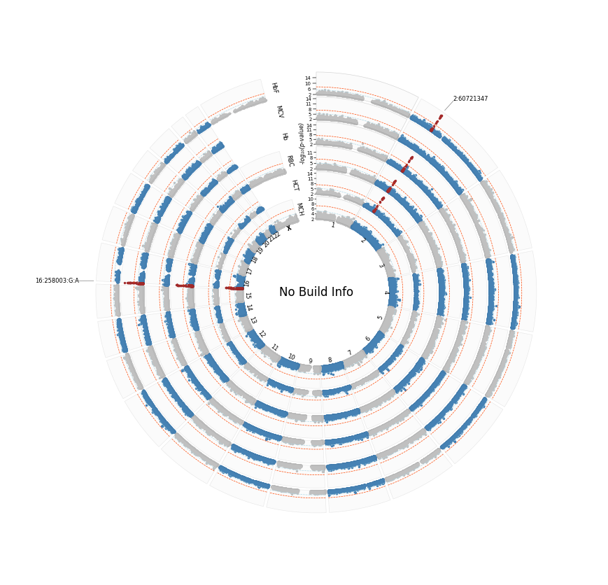
annotateis set,label_colis set, but annot_df does not contain gene information. The package defaults to ‘SNP’ column.
## Supplying builds with summary stats
[7]:
# susmtats
sumstats_no_build_col_list = [
    "/data/awonkam1/kesoh/gwas/sitt/sumher/kgp/nHbF/kgp-r2-0.60-maf-0.01_nHbF_agecut-5_kvik1.step2.assoc.gz",
    "/data/awonkam1/kesoh/gwas/sitt/sumher/h3a/nMCV/h3a-r2-0.60-maf-0.01_nMCV_agecut-5_kvik1.step2.assoc.gz",
    "/data/awonkam1/kesoh/gwas/sitt/sumher/gmv2p1/nHb/gmv2p1-r2-0.60-maf-0.01_nHb_agecut-5_kvik1.step2.assoc.gz",
    "/data/awonkam1/kesoh/gwas/sitt/sumher/gmv2p2/nRBC/gmv2p2-r2-0.60-maf-0.01_nRBC_agecut-5_kvik1.step2.assoc.gz",
    "/data/awonkam1/kesoh/gwas/sitt/sumher/caapa/nHCT/caapa-r2-0.60-maf-0.01_nHCT_agecut-5_kvik1.step2.assoc.gz",
    "/data/awonkam1/kesoh/gwas/sitt/sumher/topmed/nMCH/topmed-r2-0.60-maf-0.01_nMCH_agecut-5_kvik1.step2.assoc.gz"
]

# labels, same order as sumstatst
label_list = [
    "HbF",
    "MCV",
    "Hb",
    "RBC",
    "HCT",
    "MCH"
]

# supplying sumstat builds, same order as sumstatst and labels
build_list = [
    "hg19",
    "hg38",
    "hg19",
    "hg38",
    "hg19",
    "hg38"
]
[8]:
sumstats_info_dict = prep_pycmplot_input_info(
    sum_stats=sumstats_no_build_col_list,
    labels=label_list,
    build_list=build_list
)

sumstats_info_dict
[8]:
{'HbF': [['Chromosome', 'Basepair', 'Predictor', 'Wald_P'],
  {'Chromosome': 'category',
   'Basepair': object,
   'Predictor': str,
   'Wald_P': float},
  {'Chromosome': 'CHR', 'Basepair': 'POS', 'Predictor': 'SNP', 'Wald_P': 'P'},
  '\t',
  'hg19'],
 'MCV': [['Chromosome', 'Basepair', 'Predictor', 'Wald_P'],
  {'Chromosome': 'category',
   'Basepair': object,
   'Predictor': str,
   'Wald_P': float},
  {'Chromosome': 'CHR', 'Basepair': 'POS', 'Predictor': 'SNP', 'Wald_P': 'P'},
  '\t',
  'hg38'],
 'Hb': [['Chromosome', 'Basepair', 'Predictor', 'Wald_P'],
  {'Chromosome': 'category',
   'Basepair': object,
   'Predictor': str,
   'Wald_P': float},
  {'Chromosome': 'CHR', 'Basepair': 'POS', 'Predictor': 'SNP', 'Wald_P': 'P'},
  '\t',
  'hg19'],
 'RBC': [['Chromosome', 'Basepair', 'Predictor', 'Wald_P'],
  {'Chromosome': 'category',
   'Basepair': object,
   'Predictor': str,
   'Wald_P': float},
  {'Chromosome': 'CHR', 'Basepair': 'POS', 'Predictor': 'SNP', 'Wald_P': 'P'},
  '\t',
  'hg38'],
 'HCT': [['Chromosome', 'Basepair', 'Predictor', 'Wald_P'],
  {'Chromosome': 'category',
   'Basepair': object,
   'Predictor': str,
   'Wald_P': float},
  {'Chromosome': 'CHR', 'Basepair': 'POS', 'Predictor': 'SNP', 'Wald_P': 'P'},
  '\t',
  'hg19'],
 'MCH': [['Chromosome', 'Basepair', 'Predictor', 'Wald_P'],
  {'Chromosome': 'category',
   'Basepair': object,
   'Predictor': str,
   'Wald_P': float},
  {'Chromosome': 'CHR', 'Basepair': 'POS', 'Predictor': 'SNP', 'Wald_P': 'P'},
  '\t',
  'hg38']}
[9]:
%%time
pycmplot_dict = get_sumstats_and_merged_sector_list(
    sum_stats=sumstats_no_build_col_list,
    labels=label_list,
    file_info=sumstats_info_dict,
    logp=True,
    table_out="with_build_info",
    trim_pval=0.001,
    signif_threshold=1e-7,
)
[INFO] Loading MCV from /data/awonkam1/kesoh/gwas/sitt/sumher/h3a/nMCV/h3a-r2-0.60-maf-0.01_nMCV_agecut-5_kvik1.step2.assoc.gz …
[INFO] Loaded 12070968 variants from summary stat file, using 98.6 MB of memory
[INFO] Extracting raw p-values for QQ-plotting ...
[INFO] Excluding variants with p-value less than 0.001 to speed up Manhattan plotting ...
[INFO] 12873 variants remain after trimming, using 0.117 MB of memory
[INFO] Adding a 'logP' column ...
[INFO] Normalizing chromosome names {"23": "X", "24": "Y", "M": "MT", "MTDNA": "MT"} ...
[INFO] Extracting variants to highlight ...
[INFO] Loading HbF from /data/awonkam1/kesoh/gwas/sitt/sumher/kgp/nHbF/kgp-r2-0.60-maf-0.01_nHbF_agecut-5_kvik1.step2.assoc.gz …
[INFO] Loaded 12198661 variants from summary stat file, using 94.7 MB of memory
[INFO] Extracting raw p-values for QQ-plotting ...
[INFO] Excluding variants with p-value less than 0.001 to speed up Manhattan plotting ...
[INFO] 13741 variants remain after trimming, using 0.119 MB of memory
[INFO] Adding a 'logP' column ...
[INFO] Normalizing chromosome names {"23": "X", "24": "Y", "M": "MT", "MTDNA": "MT"} ...
[INFO] Converting hg19 coordinates to hg38 ...
[INFO] Loading LiftOver chain file: /home/kesohku1/projects/gwas/scripts/pycmplot/pycmplot/data/hg19ToHg38.over.chain.gz
[INFO] Extracting variants to highlight ...
[INFO] Loading Hb from /data/awonkam1/kesoh/gwas/sitt/sumher/gmv2p1/nHb/gmv2p1-r2-0.60-maf-0.01_nHb_agecut-5_kvik1.step2.assoc.gz …
[INFO] Loaded 12863787 variants from summary stat file, using 99.9 MB of memory
[INFO] Extracting raw p-values for QQ-plotting ...
[INFO] Excluding variants with p-value less than 0.001 to speed up Manhattan plotting ...
[INFO] 12505 variants remain after trimming, using 0.108 MB of memory
[INFO] Adding a 'logP' column ...
[INFO] Normalizing chromosome names {"23": "X", "24": "Y", "M": "MT", "MTDNA": "MT"} ...
[INFO] Converting hg19 coordinates to hg38 ...
[INFO] Extracting variants to highlight ...
[INFO] Loading RBC from /data/awonkam1/kesoh/gwas/sitt/sumher/gmv2p2/nRBC/gmv2p2-r2-0.60-maf-0.01_nRBC_agecut-5_kvik1.step2.assoc.gz …
[INFO] Loaded 13848274 variants from summary stat file, using 1.07 GB of memory
[INFO] Extracting raw p-values for QQ-plotting ...
[INFO] Excluding variants with p-value less than 0.001 to speed up Manhattan plotting ...
[INFO] 14201 variants remain after trimming, using 0.122 MB of memory
[INFO] Adding a 'logP' column ...
[INFO] Normalizing chromosome names {"23": "X", "24": "Y", "M": "MT", "MTDNA": "MT"} ...
[INFO] Extracting variants to highlight ...
[INFO] Loading MCH from /data/awonkam1/kesoh/gwas/sitt/sumher/topmed/nMCH/topmed-r2-0.60-maf-0.01_nMCH_agecut-5_kvik1.step2.assoc.gz …
[INFO] Loaded 13896844 variants from summary stat file, using 1.07 GB of memory
[INFO] Extracting raw p-values for QQ-plotting ...
[INFO] Excluding variants with p-value less than 0.001 to speed up Manhattan plotting ...
[INFO] 14008 variants remain after trimming, using 0.121 MB of memory
[INFO] Adding a 'logP' column ...
[INFO] Normalizing chromosome names {"23": "X", "24": "Y", "M": "MT", "MTDNA": "MT"} ...
[INFO] Extracting variants to highlight ...
[INFO] Loading HCT from /data/awonkam1/kesoh/gwas/sitt/sumher/caapa/nHCT/caapa-r2-0.60-maf-0.01_nHCT_agecut-5_kvik1.step2.assoc.gz …
[INFO] Loaded 4921533 variants from summary stat file, using 38.2 MB of memory
[INFO] Extracting raw p-values for QQ-plotting ...
[INFO] Excluding variants with p-value less than 0.001 to speed up Manhattan plotting ...
[INFO] 4968 variants remain after trimming, using 43.2 MB of memory
[INFO] Adding a 'logP' column ...
[INFO] Normalizing chromosome names {"23": "X", "24": "Y", "M": "MT", "MTDNA": "MT"} ...
[INFO] Converting hg19 coordinates to hg38 ...
[INFO] Extracting variants to highlight ...
[INFO] Loading gene info from: /home/kesohku1/projects/gwas/scripts/pycmplot/pycmplot/data/Homo_sapiens.GRCh38.geneinfo.tsv.gz
[INFO] Annotating lead variants and generating hits summary table ...
[INFO] Locus summary written to: with_build_info.tsv
[INFO] Computing per-sumstat sector sizes (chrom → [min_pos, max_pos])
CPU times: user 2min 16s, sys: 5.15 s, total: 2min 21s
Wall time: 2min 22s
[10]:
sectors_sizes = pycmplot_dict["sectors"]
sumstast_loaded = pycmplot_dict["dfs"]
annot_df = pycmplot_dict["annot"]
sig_lines = pycmplot_dict["lines"]
pval_dict = pycmplot_dict["pvals"]
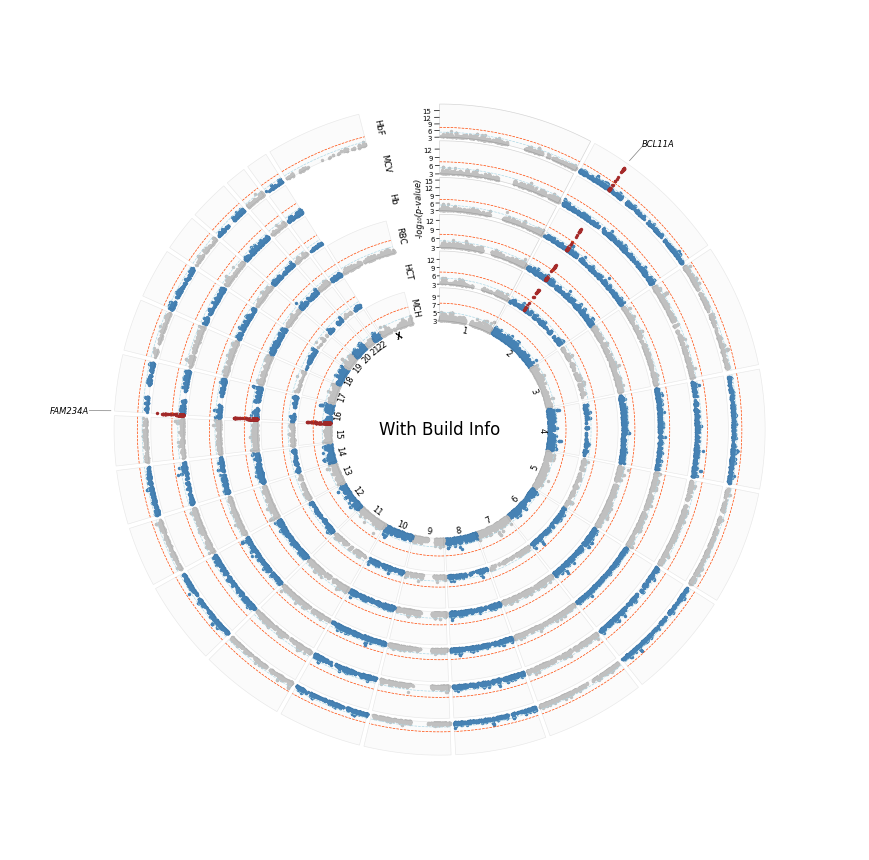
[12]:
annot_df
[12]:
| CHR | SNP | POS | P | BUILD | logP | LABEL | OLD_POS | OLD_BUILD | genic | ... | promoter_upstream_flag | gene_density | top_gene | biotype | priority_score | distance | promoter_flag | distance_score | biotype_weight | promoter_bonus | |
|---|---|---|---|---|---|---|---|---|---|---|---|---|---|---|---|---|---|---|---|---|---|
| 1 | 2 | 2:60721347 | 60494212 | 1.567800e-16 | hg38 | 15.804709 | HbF | 60721347.0 | hg19 | True | ... | False | 46 | BCL11A | protein_coding | 4.0 | 0 | False | 1.0 | 1.0 | 0.0 |
| 0 | 16 | 16:258003:G:A | 258003 | 1.094200e-13 | hg38 | 12.960903 | MCV | NaN | NaN | True | ... | False | 150 | FAM234A | protein_coding | 4.0 | 0 | False | 1.0 | 1.0 | 0.0 |
2 rows × 24 columns
[13]:
sumstast_loaded.keys()
[13]:
dict_keys(['HbF', 'MCV', 'Hb', 'RBC', 'HCT', 'MCH'])
[14]:
%%time
plot_circular(
    sumstats_loaded=sumstast_loaded,
    sector_sizes=sectors_sizes,
    annotate='gene', # remember there was no build info hence hits table was not annotated with genes. Let's see plotting behaviour in this scenario
    label_col='top_gene',
    logp=True,
    highlight=True,
    hits_table=annot_df,
    plot_title="With Build Info",
    r_min=30
)
[INFO] Plotting : HbF
[INFO] Plotting : MCV
[INFO] Plotting : Hb
[INFO] Plotting : RBC
[INFO] Plotting : HCT
[INFO] Plotting : MCH
[INFO] Annotating by: top_gene
[INFO] Saved circular Manhattan plot: /home/kesohku1/projects/gwas/scripts/pycmplot/with_build_info_hbf_mcv_hb_rbc_hct_mch_cm_logp.png
CPU times: user 7.23 s, sys: 1.27 s, total: 8.5 s
Wall time: 7.1 s
## QQ-Plotting
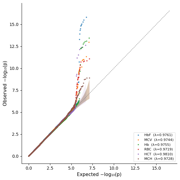
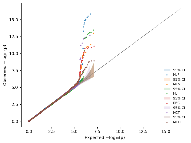
Overlaying multiple
Use
thinto speed up plotting. Otherwise, using all variants is extremely slow.By setting
thin_below, you apply thinning to only variants with p-value >= the value set. That is near the null base.
[6]:
pval_dict
[6]:
{'HbF': array([0.80238 , 0.1593  , 0.70696 , ..., 0.10506 , 0.044299, 0.044299]),
 'MCV': array([0.43549 , 0.38235 , 0.23061 , ..., 0.24768 , 0.7078  , 0.015747]),
 'Hb': array([0.36697, 0.84087, 0.84771, ..., 0.91971, 0.7597 , 0.61939]),
 'RBC': array([0.46497, 0.10017, 0.34216, ..., 0.98986, 0.33426, 0.4835 ]),
 'HCT': array([0.66248, 0.96457, 0.79573, ..., 0.38697, 0.64664, 0.55925]),
 'MCH': array([0.94428, 0.96713, 0.86231, ..., 0.35127, 0.4025 , 0.38731])}
[7]:
%%time
plot_qq_overlay(pval_dict=pval_dict, thin=True, thin_below=0.001)
[INFO] Saved combined QQ plot: None.png
[7]:
(<Figure size 600x600 with 1 Axes>,
 <Axes: xlabel='Expected −log₁₀(p)', ylabel='Observed −log₁₀(p)'>)
Separate qq-plots saved in separate figures
As ‘png’ and ‘pdf’
[11]:
%%time
# png
plot_qq_separate(
    pval_dict=pval_dict,
    thin=True,
    thin_below=0.001,
    output_path="/home/kesohku1/projects/gwas/scripts/figs/",
    base_name="test",
)

# pdf rasterized: low memory
plot_qq_separate(
    pval_dict=pval_dict,
    thin=True,
    thin_below=0.001,
    output_path="/home/kesohku1/projects/gwas/scripts/figs/",
    base_name="test_rasterized",
    fig_format='pdf',
    rasterized=True,
)

# pdf not rasterized: higher memory
plot_qq_separate(
    pval_dict=pval_dict,
    thin=True,
    thin_below=0.001,
    output_path="/home/kesohku1/projects/gwas/scripts/figs/",
    base_name="test_not_rasterized",
    fig_format='pdf',
    rasterized=False,
)
[INFO] Saved QQ plot: /home/kesohku1/projects/gwas/scripts/figs/test_HbF_MCV_Hb_RBC_HCT_MCH_qq_pval_HbF.png
[INFO] Saved QQ plot: /home/kesohku1/projects/gwas/scripts/figs/test_HbF_MCV_Hb_RBC_HCT_MCH_qq_pval_MCV.png
[INFO] Saved QQ plot: /home/kesohku1/projects/gwas/scripts/figs/test_HbF_MCV_Hb_RBC_HCT_MCH_qq_pval_Hb.png
[INFO] Saved QQ plot: /home/kesohku1/projects/gwas/scripts/figs/test_HbF_MCV_Hb_RBC_HCT_MCH_qq_pval_RBC.png
[INFO] Saved QQ plot: /home/kesohku1/projects/gwas/scripts/figs/test_HbF_MCV_Hb_RBC_HCT_MCH_qq_pval_HCT.png
[INFO] Saved QQ plot: /home/kesohku1/projects/gwas/scripts/figs/test_HbF_MCV_Hb_RBC_HCT_MCH_qq_pval_MCH.png
[INFO] Saved QQ plot: /home/kesohku1/projects/gwas/scripts/figs/testrasterized_HbF_MCV_Hb_RBC_HCT_MCH_qq_pval_HbF.pdf
[INFO] Saved QQ plot: /home/kesohku1/projects/gwas/scripts/figs/testrasterized_HbF_MCV_Hb_RBC_HCT_MCH_qq_pval_MCV.pdf
[INFO] Saved QQ plot: /home/kesohku1/projects/gwas/scripts/figs/testrasterized_HbF_MCV_Hb_RBC_HCT_MCH_qq_pval_Hb.pdf
[INFO] Saved QQ plot: /home/kesohku1/projects/gwas/scripts/figs/testrasterized_HbF_MCV_Hb_RBC_HCT_MCH_qq_pval_RBC.pdf
[INFO] Saved QQ plot: /home/kesohku1/projects/gwas/scripts/figs/testrasterized_HbF_MCV_Hb_RBC_HCT_MCH_qq_pval_HCT.pdf
[INFO] Saved QQ plot: /home/kesohku1/projects/gwas/scripts/figs/testrasterized_HbF_MCV_Hb_RBC_HCT_MCH_qq_pval_MCH.pdf
[INFO] Saved QQ plot: /home/kesohku1/projects/gwas/scripts/figs/testnotrasterized_HbF_MCV_Hb_RBC_HCT_MCH_qq_pval_HbF.pdf
[INFO] Saved QQ plot: /home/kesohku1/projects/gwas/scripts/figs/testnotrasterized_HbF_MCV_Hb_RBC_HCT_MCH_qq_pval_MCV.pdf
[INFO] Saved QQ plot: /home/kesohku1/projects/gwas/scripts/figs/testnotrasterized_HbF_MCV_Hb_RBC_HCT_MCH_qq_pval_Hb.pdf
[INFO] Saved QQ plot: /home/kesohku1/projects/gwas/scripts/figs/testnotrasterized_HbF_MCV_Hb_RBC_HCT_MCH_qq_pval_RBC.pdf
[INFO] Saved QQ plot: /home/kesohku1/projects/gwas/scripts/figs/testnotrasterized_HbF_MCV_Hb_RBC_HCT_MCH_qq_pval_HCT.pdf
[INFO] Saved QQ plot: /home/kesohku1/projects/gwas/scripts/figs/testnotrasterized_HbF_MCV_Hb_RBC_HCT_MCH_qq_pval_MCH.pdf
[11]:
['/home/kesohku1/projects/gwas/scripts/figs/testnotrasterized_HbF_MCV_Hb_RBC_HCT_MCH_qq_pval_HbF.pdf',
 '/home/kesohku1/projects/gwas/scripts/figs/testnotrasterized_HbF_MCV_Hb_RBC_HCT_MCH_qq_pval_MCV.pdf',
 '/home/kesohku1/projects/gwas/scripts/figs/testnotrasterized_HbF_MCV_Hb_RBC_HCT_MCH_qq_pval_Hb.pdf',
 '/home/kesohku1/projects/gwas/scripts/figs/testnotrasterized_HbF_MCV_Hb_RBC_HCT_MCH_qq_pval_RBC.pdf',
 '/home/kesohku1/projects/gwas/scripts/figs/testnotrasterized_HbF_MCV_Hb_RBC_HCT_MCH_qq_pval_HCT.pdf',
 '/home/kesohku1/projects/gwas/scripts/figs/testnotrasterized_HbF_MCV_Hb_RBC_HCT_MCH_qq_pval_MCH.pdf']
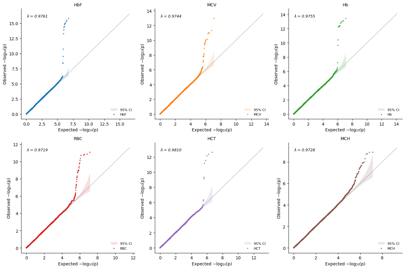
Combined multi-panel
[12]:
%%time
plot_qq_combined(pval_dict=pval_dict, thin=True, thin_below=0.001)
[12]:
(<Figure size 1350x900 with 6 Axes>,
 [<Axes: title={'center': 'HbF'}, xlabel='Expected −log₁₀(p)', ylabel='Observed −log₁₀(p)'>,
  <Axes: title={'center': 'MCV'}, xlabel='Expected −log₁₀(p)', ylabel='Observed −log₁₀(p)'>,
  <Axes: title={'center': 'Hb'}, xlabel='Expected −log₁₀(p)', ylabel='Observed −log₁₀(p)'>,
  <Axes: title={'center': 'RBC'}, xlabel='Expected −log₁₀(p)', ylabel='Observed −log₁₀(p)'>,
  <Axes: title={'center': 'HCT'}, xlabel='Expected −log₁₀(p)', ylabel='Observed −log₁₀(p)'>,
  <Axes: title={'center': 'MCH'}, xlabel='Expected −log₁₀(p)', ylabel='Observed −log₁₀(p)'>])
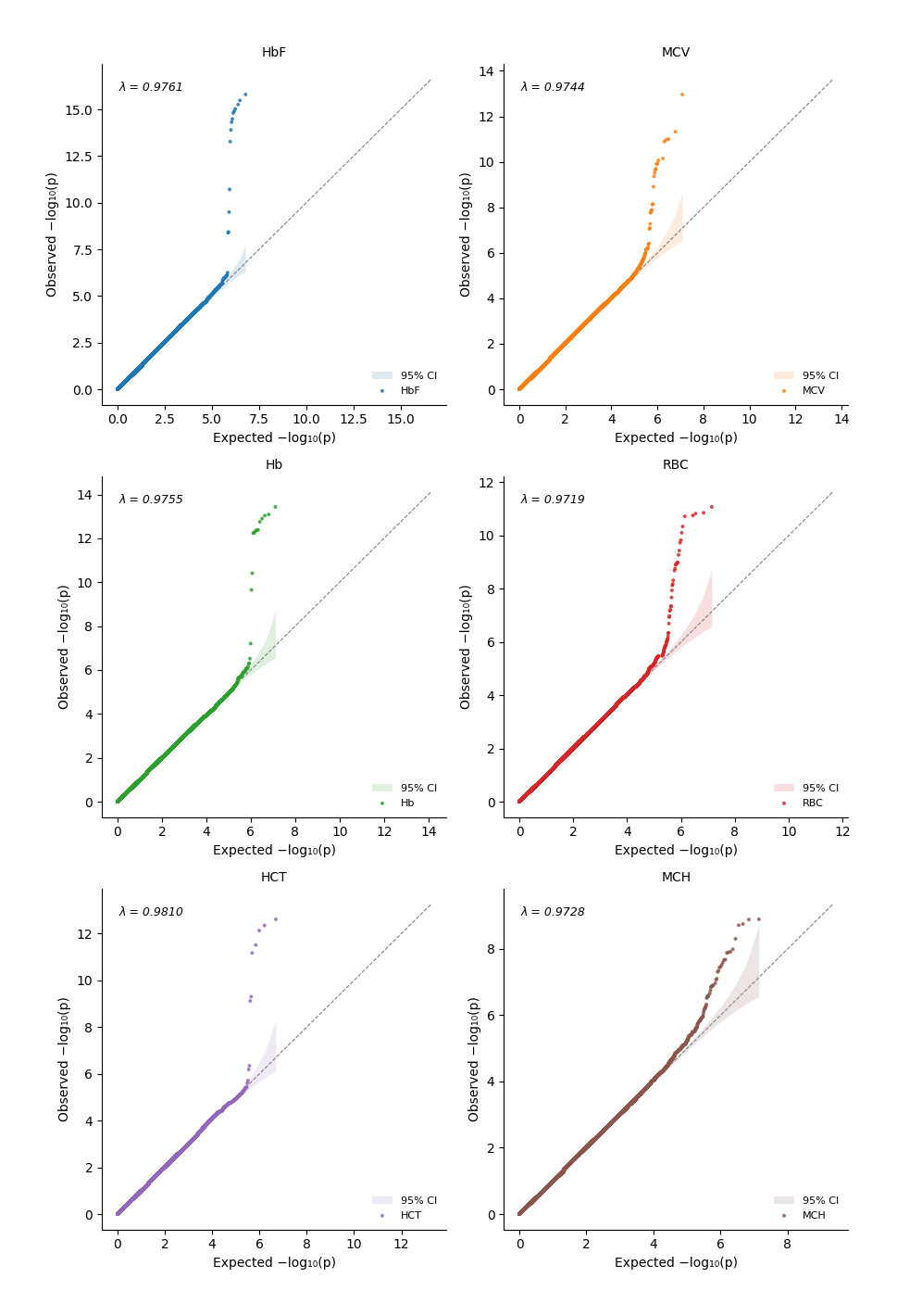
Customizing the grid arrangement
Use
ncols(number of columns)
[41]:
%%time
plot_qq_combined(pval_dict=pval_dict, thin=True, thin_below=0.001, ncols=2)
[41]:
(<Figure size 900x1350 with 6 Axes>,
 [<Axes: title={'center': 'HbF'}, xlabel='Expected −log₁₀(p)', ylabel='Observed −log₁₀(p)'>,
  <Axes: title={'center': 'MCV'}, xlabel='Expected −log₁₀(p)', ylabel='Observed −log₁₀(p)'>,
  <Axes: title={'center': 'Hb'}, xlabel='Expected −log₁₀(p)', ylabel='Observed −log₁₀(p)'>,
  <Axes: title={'center': 'RBC'}, xlabel='Expected −log₁₀(p)', ylabel='Observed −log₁₀(p)'>,
  <Axes: title={'center': 'HCT'}, xlabel='Expected −log₁₀(p)', ylabel='Observed −log₁₀(p)'>,
  <Axes: title={'center': 'MCH'}, xlabel='Expected −log₁₀(p)', ylabel='Observed −log₁₀(p)'>])
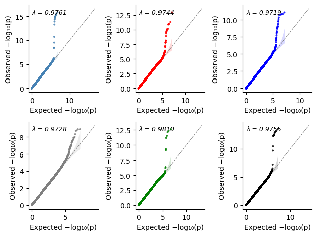
Flexible handling of each qq-plot using the base plot_qq_single function directly
Define your own axes
Pass them to
axparameter
[13]:
%%time
import matplotlib.pyplot as plt

fig, axs = plt.subplots(2,3, squeeze=False)

plot_qq_single(thin=True, thin_below=0.001, pvals=pval_dict["HbF"], ax=axs[0][0], ci=0.95, show_lambda=True)
plot_qq_single(thin=True, thin_below=0.001, pvals=pval_dict["MCV"], ax=axs[0][1], ci=0.95, show_lambda=True, color="red")
plot_qq_single(thin=True, thin_below=0.001, pvals=pval_dict["RBC"], ax=axs[0][2], ci=0.95, show_lambda=True, color="blue")
plot_qq_single(thin=True, thin_below=0.001, pvals=pval_dict["MCH"], ax=axs[1][0], ci=0.95, show_lambda=True, color="grey")
plot_qq_single(thin=True, thin_below=0.001, pvals=pval_dict["HCT"], ax=axs[1][1], ci=0.95, show_lambda=True, color="green")
plot_qq_single(thin=True, thin_below=0.001, pvals=pval_dict["Hb"], ax=axs[1][2], ci=0.95, show_lambda=True, color="black")

plt.tight_layout()
Or overlay them by simply using the same axis
[22]:
%%time
import matplotlib.pyplot as plt
import matplotlib.colors as mcolors

# We will need separate colors for the sumstats
labels = pval_dict.keys()
n = len(labels)
cmap = plt.get_cmap("tab10")
colors = [mcolors.to_hex(cmap(i % 10)) for i in range(n)]

fig, axs = plt.subplots()

for label, color in zip(labels, colors):
    plot_qq_single(
        thin=True,
        thin_below=0.001,
        pvals=pval_dict[label],
        ax=axs,
        ci=0.95,
        label=label,
        color=color,
        show_lambda=False, # However, `plot_qq_overlay` and `plot_qq_combined` handle `show_lambda` better.
    )

plt.tight_layout()
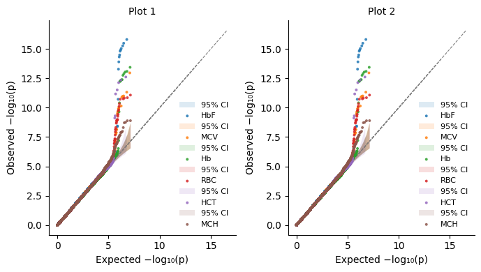
This gives us the flexibility to place multiple overlay plots on one figure
[28]:
%%time
import matplotlib.pyplot as plt
import matplotlib.colors as mcolors

# We will need separate colors for the sumstats
labels = pval_dict.keys()
n = len(labels)
cmap = plt.get_cmap("tab10")
colors = [mcolors.to_hex(cmap(i % 10)) for i in range(n)]

fig, axs = plt.subplots(1, 2, squeeze=False, figsize=(7,4))

for label, color in zip(labels, colors):
    plot_qq_single(
        thin=True,
        thin_below=0.001,
        pvals=pval_dict[label],
        ax=axs[0][0],
        ci=0.95,
        label=label,
        color=color,
        title="Plot 1",
        show_lambda=False, # However, `plot_qq_overlay` and `plot_qq_combined` handle `show_lambda` better.
    )

for label, color in zip(labels, colors):
    plot_qq_single(
        thin=True,
        thin_below=0.001,
        pvals=pval_dict[label],
        ax=axs[0][1],
        ci=0.95,
        label=label,
        color=color,
        title="Plot 2",
        show_lambda=False, # However, `plot_qq_overlay` and `plot_qq_combined` handle `show_lambda` better.
    )
plt.tight_layout()
# Final Notes
The
prep_pycmplot_input_infofunction saves the hits table as a TAB delimited file (.tsv) with the plot title provided combined with the labels and type of plot (lm or cm).If plot title is not provided, the function generates a random string for the file name and plot name.
All files are saved in the user provided output directory using
output_dir. If not provided, the current directory'.'is used.